Search is a key part of many Artificial Intelligence (AI) problem-solving strategies that assist in exploring problem spaces. As explained by Peter Norvig, “Normal programming is telling the computer what to do when we know what to do. AI is when we tell the computer what to do when we don’t know what to do.”
Search in AI is the first step to start solving many of the problems; either by finding a sequence of the next steps for an agent to perform or by deciding the next game move.
Many search strategies are used in AI for efficient and goal-oriented searches. Let’s take a look at a few popular AI search strategies:
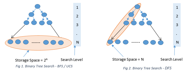
Breadth-First Search (BFS) is the most basic search and it finds the shortest path with respect to a number of steps between the start and the goal. Simple BFS does not consider any edge costs or weights. A queue with FIFO implementation can be used to keep track of the frontier of the explored nodes. BFS is undirected and will start expanding the search in all directions from the start and also complete; so it is guaranteed to find the path even in an infinite problem space. In terms of storage space, BFS will need to store 2N number of nodes in memory at any given level N, so it is expensive if the storage space is stringent, especially in larger problem spaces.
Uniform Cost Search or Cheapest First Search finds the most optimal path from start to goal with respect to the edge cost. A priority queue is used normally to get the next lowest cost node to be explored. Like BFS, a uniform cost search is undirected, complete, and guarantees to find the optimal solution. More or less, it also requires a storage space of 2N.
Depth First Search (DFS) finds the longest path from the start. It is non-optimal and can find the way to a goal, but it might not be the most optimal way to reach the goal. DFS is also not complete. If it gets into an infinite path, it is very likely that it will never reach the goal. However, it does have an advantage in terms of storage space. DFS will need to store only N nodes of the current path. This is a winner when the problem space is very big and space is a constraint. Figure 1 and Figure 2 below illustrate the difference between BFS and DFS for a binary tree search.
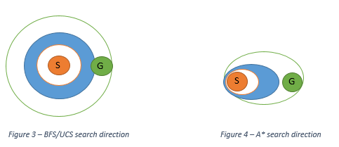
A* search is a directed search towards the goal. It expands the path in the direction that has the minimum cost and minimum estimated distance towards the goal. It is like adding a little bit of more knowledge to the uniform cost algorithm so that it explores lesser number of nodes to find the optimal path. The estimated distance can be any heuristic such as the direct distance between the node and the goal node. For A* to find the optimal path, the heuristic value should be less than the true value of the cost for that path. That is, it should never overestimate the true cost.
Figure 3 and Figure 4 below show contour maps for the nodes explored in BFS/UCS and A* and the direction in which they are explored from the start to the goal nodes.
All the aforementioned search strategies are helpful when we are trying to find a sequence of steps such as finding out the best possible routes between 2 cities, finding the next step in solving the rubric’s cube. Some AI problems also deal with plotting against another AI agent or a human. As in game playing, the AI agent needs to anticipate the move of the opposition player and then search for the most optimal move from the game tree.
Adversarial searches are when the AI agents anticipate and plan ahead of other agents.
The Minimax Search Algorithm is an adversarial search algorithm. In this algorithm, we choose the best moves to maximize the chances to win, assuming that the opponent is also playing optimally to win, minimizing our chances. For every action taken by the opponent, all the possible actions remaining are evaluated using a game tree till the end game. The win values are propagated as positive when our agent wins and negative when the opponent wins to the top of the tree. At every level where our agent plays (max level), it selects the branch with the max value. At every level the opponent plays (min level), it selects the branch with the min value. The algorithm tries to choose the moves that lead to a win for our agent.
Even for very less complicated games or situations, the minimax tree will approximately visit an exponential number of nodes when evaluated till the end game. For a tree with a branching factor of b and depth of d, the minimax tree needs to visit bd nodes approximately. Most of the situations in AI need the agent to be very responsive. So, implementing minimax till the end game is very expensive.
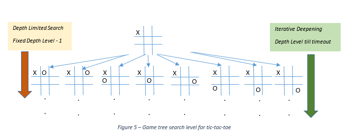
The Depth Limited Search is normally used along with an evaluation function when implementing minimax. In this case, we calculate how deep in the game tree the agent searches before response limit timeout. So, we calculate the N level for which the agent searches safely. At the Nth level, the agent uses an evaluation function, which is an estimated measure of the win value of the game. Say, for a game of tic-tac-toe, it can be the number of moves remaining for the agent. An agent with more moves remaining will mostly win. The value of the evaluation function is then propagated to the top of the tree to calculate the best move.
Iterative Deepening is one more strategy where the agent at every level saves the best move calculated. Then, it again starts from the top of the tree and tries to search for the next level. It keeps on searching deeper in the tree until it reaches the response timeout. Then it returns the last saved move for a completely evaluated level. So, it is similar to depth limited search, but it continues searching deeper till time remains. It is particularly useful near the end of the game where the branching factor reduces significantly and the agents can search at deeper levels.
Figure 5 illustrates the search level for depth limited and iterative deepening techniques.
The Alpha Beta Pruning technique is yet another strategy that ignores a lot of branches in minimax and yet returns exactly the same result as the minimax algorithm. It ignores moves that return less than maximum values at max levels where our agent takes any action. At min levels of a tree where an opponent chooses, it ignores moves that have more than min values at that level. This reduces the number of nodes to be evaluated as much as bd/2 in some cases when the best move node ordering is done.
Different search strategies are applied in AI depending on the problem type, the resources available, and the applicability of the strategy. A few popular ones are described above.
References:
“Artificial Intelligence: A modern approach”, Third Edition, By Peter Norvig & Stuart Russell


